
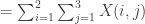
Lesson 1: 基礎 Python
Objective:
- 學習進入 Python 計算的基礎語法與指令。
- 學習安裝套件、使用模組,譬如數學相關的 numpy 、統計計算相關的 scipy、繪圖相關的 matplotlib
Prerequisite:
- 安裝 Python 與 Visual Studio Code (IDE) + Jupyter Notebook extensions 及其他客製化的 extensions。
- 熟悉在 Jupyter Notebook 的 markdown 技術,寫
數學式及其他文字表現。
- 欣賞一些 Python 寫作技巧:
範例 0:在 IDE(Integrated Development Environment, e.g. VS Code)建立虛擬環境(Virtual Environment)
說明:
甚麼是虛擬環境?去問問 ChatGPT。
為何需要在 IDE 建立虛擬環境?有何好處?有何缺點?
如何建立虛擬環境?(以下步驟必須詳細說明方能理解)
虛擬環境將被設置在一個子目錄裡,假設目錄名稱為 venv_name
建立虛擬環境的命令:python -m venv venv_name
從 vscode 重新進入目錄(Open Folder) venv_name,選擇以 venv_name 為名的 Python interpreter。
開始在虛擬環境下寫程式。
建立虛擬環境可能遇到作業系統的安全問題,解決方式與步驟如下圖。
以「系統管理員身分執行」 Power Shell
執行指令: Get-ExecutionPolicy -List
在 LocalMachine 項目的 ExecutionPolicy 必須是 RemoteSigned
如果不是,則執行指令 Set-ExecutionPolicy -ExecutionPolicy RemoteSigned
回應系統安全說明並變更執行原則: Y

以下範例僅供參考,不是唯一的做法,也不一定是最好的做法。Python 是自由軟體,各種功能的指令多到不可數計,除常用指令另外,很難記住所有指令。因此寫程式時,可以依賴 chatGPT 的協助,其中以與 vscode 搭配的 GitHub copilot 的 inline coding 效率最高,能即時、自動地提供適當的指令,不論對新手或老手幫助都甚大。目前加入 GitHub 的學生與老師會員,能免費使用 copilot。下圖展示在 vscode insiders (vscode 的隱藏版本)環境下,安裝了 GitHub copilot 後的樣子。其中右下角的小圖案代表成功安裝了 copilot,中間呈現了 copilot 的 inline coding 的功能,能自動猜測程式即將進行的功能,並浮現出灰色程式碼,等待接受與否。最左邊的後面的小圖,代表安裝了 GitHub copilot chat,可以在左邊開出視窗進行 chatGPT 的問答。此時的問答將會根據右邊的程式碼,甚至該目錄的程式碼內容回應,答案往往較能滿足程式員的需求。

範例 1: Python 的數字(number), 向量(vector) 與矩陣(array)
注意事項:
如果沒有建立虛擬環境,建議建立一個全新的目錄,並在 VS Code 中開啟 folder,然後建立一個新檔案,檔名 lesson_1.py。輸入下列每個範例的每一行指令,執行並觀察結果。
在 VS Code 中執行副檔名為 py 的程式,執行的目標地點為下方的 terminal 視窗。而且除非使用 print(變數名稱),否則看不到執行結果。
另一個執行方式是借用 Jupyter Notebook 的延伸功能,將程式執行交給 Jupyter Notebook。 做法如下:
在程式上輸入 #%% 將在上一行產生如圖一的一排執行工具,將程式切割為以 cell 為執行單位。選擇「Run Cell」執行 cell 內的程式碼,此時除了在右邊新增一 Jupyter 互動視窗顯示並執行結果外,在下面的 terminal 視窗也會多出一個「Jupyter Variables」的選項,裡面呈現目前為止出現過的變數名稱,及其資料形態與內容。方便觀察變數內容,不一定要用 print()。
第一次以 Jupuyter Notebook 的方式執行 cell 程式碼時, VS Code 會自動通知安裝套件「ipykernel」,安裝後即可執行。
以上陳述針對以 py 為副檔名的程式,若有互動的需要才這樣做,並非常態性作法。一般對 py 檔都是直些執行,讓結果顯示在下面的 Terminal 視窗,圖形從新視窗產生。若需要 Jupyter Notebook 的互動式功能,可以選擇附檔名 ipynb,如圖二,便可以使用 Jupyter Notebook 的全功能,包括 Markdown淤的編輯功能。 執行後,可以從 JUPYTER VARIABLES 看到每個變數的內容。
下列的指令與語法的學習,採猜測的原則(從已經熟悉的某個語言)。從執行的結果去驗證。若還猜不到,可以上網查詢官網的說明。
變數名稱盡量能自我說明,長一點無所謂。
Python 程式的格式有一定的樣子,可以使用 VS Code 的功能「Format Document」(按右鍵),程式碼會自動調整為較符合 coding 的原則。
#%% 1. Numbers

int_number = 1
float_number = 1.0
complex_number = 1 + 2j
round_float = round(1234.5678, 2)
str2int = int('213')

print(round_float)

number_list = [0, 1, 1, 2, 3, 5, 8]
slicing_4_a_specific_pos = number_list[3]
slicing_4_the_last_pos = number_list[-1]
slicing_4_consecutive_pos = number_list[0:3]
slicing_4_the_last_three = number_list[-3:]

list_list = [[1, 2, 3], [4, 5, 6]]  # list of list
A_list = list_list[0]
A_ist_list = list_list[0:2]
A_number = list_list[1][2]

注意事項:
開始使用 numpy 套件建立矩陣。安裝方式(在下方 terminal 視窗): pip install numpy.
使用 np.size() and np.shape() 觀察矩陣或向量的大小。 若使用 Jupyter 的 ipynb 副檔名,則可以從 Jupyter Variables 裡的變數名稱看到矩陣大小的資訊,甚至可以打開觀看內容。
練習向量與矩陣(array)的區塊切片(slicing)。
# Array and slicing
import numpy as np

a = np.array([1, 2, 3]) # a vector has no direction
A = np.array([[1, 2, 3]]) # a 1 x 3 array that can be transposed
a_T = a[:, np.newaxis] # a' although a has no direction
A_T = A.T # A'
B = A.reshape(-1, 1) # A'
C = np.array([1, 2, 3], ndmin = 2) # convert a to A
print(np.size(a))  # == print(a.size) number of elements in a
print(np.shape(A_T))  # == print(A_T.shape) , array dimension

D = np.array([[1, 2, 3],[4, 5, 6]])
print(D[1]) # D[1] = D[1,:] # second row and all columns
print(D[:, 1]) # 取第 2 行
print(D[:, :-1]) # 取前幾行,除了最後一行
print(D[:, 1:]) # 取第 2 行後所有行
print(D[:, -2:]) # 取倒數兩行
矩陣堆疊(Array concatenation)
# vector concatenation

va = np.array([1, 2, 3])
vb = np.array([4, 5, 6])
vc = np.concatenate((va, vb), axis = 0) # flatten a, b; try axis=1
vd = np.append(va, vb)
ve = np.hstack((va, vb))
vF = np.vstack((va, vb))
vg = np.r_[va, vb]
vG = np.c_[va, vb]
vH = (va, vb) # a tuple
#matrix concatenation

ma = np.array([[1, 2, 3]]) # 1 x 3
mb = np.array([[4, 5, 6]]) # 1 x 3
mc = np.hstack((ma, mb))   # 1 x 6

# Vertically, concatenate row-wisely
mC = np.concatenate((ma, mb), axis = 0) # 2 x 3
mD = np.r_[ma, mb] # 2 x 3
mE = np.vstack((ma,mb)) #2 x 3

# Horizontally, concatenate column-wisely
mF = np.concatenate((ma.T, mb.T), axis =1) # 3 x 2
mG = np.hstack((ma.T, mb.T)) # 3 x 2
mH = np.c_[ma.T, mb.T] # 3 x 2
一些矩陣操作(Array manipulations)
S = np.array([[1, 3, 2], [6, 5, 4]])
print(S)
print(S.max())
print(S.max(0)) # column max
print(np.max(S, axis = 1)) # row max

a = S.flatten() # turn into vector
b = S.flatten('F') # turn into vector column-wise
S[S < 3] = 0 # check what S looks like

c = [1, 2, 3, 4]
C = np.tile(c,(5,1)) # repeat a matrix c : 5 x 4 matrix
d = np.reshape(C, (-1, 1)) # convert to Column vector
e = np.reshape(C, (1, -1)) # convert to row vector

# array sorting
a = np.array([1, 5, 2, 7, 4])
a_sort = np.sort(a)
a_sort_idx = np.argsort(a)
a_sort_descending = np.sort(a)[::-1]
Note: The Difference Between a List and an Array in Python
Arrays and lists are both used in Python to store data, but they don’t serve exactly the same purposes. They both can be used to store any data type (real numbers, strings, etc), and they both can be indexed and iterated through, but the similarities between the two don’t go much further. The main difference between a list and an array is the functions that you can perform to them. For example, you can divide an array by 3, and each number
in the array will be divided by 3 and the result will be printed if you request it. If you try to divide a list by 3, Python will tell you that it can’t be done, and an error will be thrown. (citation: Quick Tip: The Difference Between a List and an Array in Python)
tuple
a_tuple = (0, 0) # ordered sequence
also_a_tuple = 0, 0
a_3d_tuple = (0, 1, 2) # (2,1,0) is different, however the list  [0,1,2] := [1,2,0]
Special matrices
import numpy as np

Z = np.zeros((3,4)) # 3 x 4 zero matrix
One =  np.ones((3,4)) # 3 x 4 one matrix
I = np.eye(3) # 3 x 3 identity matrix
D = np.diag([1, 2, 3, 4]) # a diagonal matrix
e = np.diag(I) # the diagonal of I
Sequencial numbers
Note: list and range type can not do math operations
import numpy as np

x0 = [1, 2, 3, 4, 5, 6, 7, 8, 9] # a list
x1 = range(1, 10, 1) # a range
x2 = np.arange(1, 10, 1)  # an array of integer numbers
x3 = np.linspace(1, 9, 9)  # an array of float number
x4 = np.arange(10)  # start from 0 to 9
x5 = np.linspace(0, 100, 1000)

y1 = x2 + x3 + 1 # not x0 + x1 + 1
y2 = x2 ** 2 + x2 - 2
y3 = x2 / x3
範例 2: Python 的字串(string)與索引(indexing, slicing)
注意事項:
一個字串等於一些字母構成的向量
#%% string & indexing

s1 = 'a single quote string'
s2 = "a double quote string"
s3 = '''a triple quote string'''

print(s3[0])
print(s2[:4])
print(s3)

s4 = """
Triple double quotes
is usually used
in multiple lines, such as documents
"""
print(s4)

# concatenate strings
s5 = 'This is ' + s1

# string list
str_list = ['r', 'g', 'b', 'k', 'y']
print(str_list[1])

# Dictionaries
meals = {'breakfast': 'sardines', 'lunch': 'salad', 'dinner': 'cake', 'cost':40}
print(meals['breakfast'])
print(meals['cost'])
print('The meal costs {} dollars'.format(meals['cost']))
String manipulatipns
col_names = ['col1', 'col2', 'col3'] # string list
col_names_join = ','.join(col_names) # convert to a string
col_names_split = col_names_join.split(',') # convert a string to a list

a_sentence = "台北大學統計系"
where_am_I = a_sentence.find('統計')
where_is_it = a_sentence.find('會計') # -1 means NOT FOUND
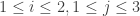
範例 3:matrix operations
Let
![X = \left[ \begin{array}{ccc} 1 & 2 & 3 \\ 4 & 5 & 6 \\ \end{array} \right] \;\;,](https://s0.wp.com/latex.php?latex=X+%3D+%5Cleft%5B+++++++++++++%5Cbegin%7Barray%7D%7Bccc%7D+++++++++++++++++1+%26+2++%26+3+%5C%5C+++++++++++++++++4+%26+5++%26+6+%5C%5C+++++++++++++%5Cend%7Barray%7D+%5Cright%5D+%5C%3B%5C%3B%2C&bg=ffffff&fg=333333&s=0&c=20201002)
![A = \left[ \begin{array}{ccc} 1 & 1 & 1 \\ 2 & 4 & 6 \\ 5 & 7 & 6 \end{array} \right]\;\;\;,](https://s0.wp.com/latex.php?latex=A+%3D+%5Cleft%5B+++++++++++++%5Cbegin%7Barray%7D%7Bccc%7D+++++++++++++++++1+%26+1++%26+1+%5C%5C+++++++++++++++++2+%26+4++%26+6+%5C%5C+++++++++++++++++5+%26+7++%26+6+++++++++++++%5Cend%7Barray%7D+%5Cright%5D%5C%3B%5C%3B%5C%3B%2C&bg=ffffff&fg=333333&s=0&c=20201002)
![b = \left[ \begin{array}{c} 1 \\ 2 \\ 3 \end{array} \right]](https://s0.wp.com/latex.php?latex=b+%3D+%5Cleft%5B+++++++++++++%5Cbegin%7Barray%7D%7Bc%7D+++++++++++++++++1++%5C%5C+++++++++++++++++2+%5C%5C+++++++++++++++++3+%5Cend%7Barray%7D+%5Cright%5D&bg=ffffff&fg=333333&s=0&c=20201002)
仔細地計算下列每一個矩陣的運算。從結果去猜測指令的意思。
-
-
for
-
for
-
- total_sum
- row_sum
- col_sum
-
-
-
-
-
, i.e. add a new row vector after the last row of A.
-
, i.e. add a new column vector after the last column of A.


from numpy import linalg
import numpy as np
import scipy.linalg as LA # scipy's linear algebra is better

X = np.array([[1,2,3],[4,5,6]]) # a 2x3 matrix
# check the information of X
Xdim = X.ndim
Xshape = X.shape
Xsize = X.size

a = X[0, 1]
P = X * X # element by element multiplication
Q = X / X # element by element division
R = X @ X.T # XX'

total_sum = X.sum() # X.mean()...
row_sum = X.sum(axis = 1) # sum over each row
col_sum = X.sum(axis = 0) # sum over each column
# col_sum = np.sum(X, axis = 0)

A = np.array([[1, 1, 1],[2, 4, 6],[5, 7, 6]])
b = np.array([1, 2, 3])
x =  LA.inv(A) @ b  # Ax = b
xsol = LA.solve(A, b) # Ax = b
I = A @ LA.inv(A) # double check what LA.inv(A) is

A_square = linalg.matrix_power(A, 2) # nth power of a matrix
A_square_root = LA.fractional_matrix_power(A, 0.5)

B = np.vstack((A, b)) # 4 x 3
C = np.hstack((A, b.reshape(3, 1))) # 3 x 4

B_row = np.insert(A, 3, b, 0) # 3 is the position index; 0 is for row
B_col = np.insert(A, 3, b, 1) # 3 is the position index; 1 is for column
範例 4:Logical operations
邏輯式運算非常好用,往往讓程式變得很簡潔。
import numpy as np

x = np.array([1, 2, 5, 3, 2])
x[x > 3] = 9 # replaced by 9; conditioned on x>3
y = np.where(x > 3, 9, x)
z = np.where(x >=3, 1, 0)
#-------------------------------
p = [] # p is a empty list
print(not p)  # check if p is empty or not
# print(p is None)
# Check whether variable p is defined or not
print('p' in locals())
#-------------------------------
a = 3
if a > 1 and a < 5 :
    print('TRUE')
else :
    print('FALSE')

if a > 5 or a < 1 :
    print('OUTSIDE')
else :
    print('INSIDE')
#-------------------------------
# compact expression for if...else...
flag = 1
status = "play" if flag ==1 else "stop"
print(status)
範例 5:Pandas dataframe basics
注意事項:
Pandas 擅長以近似 EXCEL 表格的方式處理資料,除了整理資料外(匯入、匯出),計算與繪圖也都很方便,省去許多自己 coding 的時間。
下列程式碼展現 Pandas 建立與處理資料的能力,包括:
增加欄資料、列資料與欄標題。
刪除欄資料、列資料
Create a Pandas dataframe
import pandas as pd

A = [[1,2,3,4], [5,6,7,8], [9,10,11,12]]
df = pd.DataFrame(A)
df

Add headers, add data to extend columns
df.columns = ["col1", "col2", "col3", "col4"]
c1 = [91, 92, 93]
c2 = [71, 72, 73]
c3 = [51, 52, 53]
c4 = [31, 32, 33]
df = df.assign(col5 = c1) # add c1 to the last column with header="col5"
df.insert(2, 'new', c2) # insert c2 to column#2 with header="new"
df['col6'] = c3 # add c3 to the last column with header="col6"
df

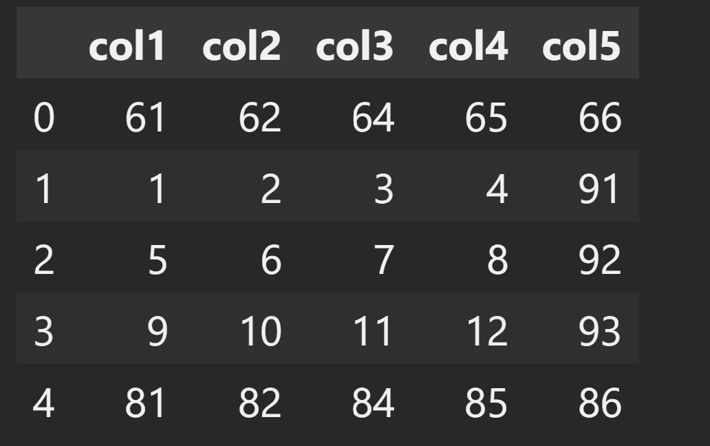
Add data to extend rows
r1 = [81, 82, 83, 84, 85, 86, 87]
df.loc[len(df)] = r1 # add r1 to the last row (the last location)
r2 = [61, 62, 63, 64, 65, 66, 67]
df.loc[-0.5] = r2 # add r2 and move to the top location
df = df.sort_index().reset_index(drop=True)
df.loc[1.5] = r2 # insert r2 in the location between row1 and row2
df = df.sort_index().reset_index(drop=True)
df

drop specified columns and rows
# 察看結果便知道下列幾行的功能
df.drop(['new', 'col6'], axis=1, inplace=True)
df.drop(df.index[2], inplace=True)
df = df.sort_index().reset_index(drop=True)
df
Slicing dataframe by row and column numbers
print(df.loc[0:3]) # loc denotes row number
print(df[["col2", "col3"]].loc[0:2])
print(df.iloc[0:3, 0:4])
D = df.values.astype(int) # convert pandas dataframe to numpy array
print(D)

範例 6:Pandas dataframe basics:檔案讀取、儲存與常見的資料處理。
注意事項:下列程式示範從網路下載 CSV 檔案,並刪除有遺失資料的部分,再改存為 XLSX 檔。
import pandas as pd

penguins_data="https://raw.githubusercontent.com/datavizpyr/data/master/palmer_penguin_species.tsv"
df = pd.read_csv(penguins_data, sep="\t")  # pd.read_excel()
df = df.dropna() # drop NA data (missing data)
print(df.head(10)) # print out the first 10 rows of data
print(df.info())
print(df.describe())
df.to_excel('pengnus_species.xlsx') # save as a xlsx file
下列程式用 pandas 開啟 XLSX 檔,並改為 numpy 的矩陣型態。
df = pd.read_excel('pengnus_species.xlsx')
np_data = np.array(df)
