SML/Lesson 9: 從 PyTorch 的淺度到深度機器學習
參考網頁文章:
- 深度學習框架: PyTorch與TensorFlow:一篇介紹兩者差異的短文。
- 機器/深度學習: 基礎介紹-損失函數(loss function) : 一篇關於機器學習的 Loss function 介紹。
- 【CNN】很詳細的講解什麼以及為什麼是卷積(Convolution)!: 圖解 Convolution 的意思。
- Example of 2D convolution: 圖像矩陣與核矩陣的卷積過程。
- PyTorch: NEURAL NETWORKS: PyTorch 官網對 CNN 的架構定義與練習。
- PyTorch: TRAINING A CLASSIFIER: PyTorch 官網的深度學習教學範例(Data: CIFAR10)。
- PyTorch Convolutional Neural Network With MNIST Dataset: 一篇使用 PyTorch CNN 辨識手寫數字的範例。
- Neural Networks in Python: From Sklearn to PyTorch and Probabilistic Neural Networks. : 從 Sklearn 的傳統神經網路 MLPClassifier 到 PyTorch 的 CNN 網路,到自訂的貝氏機率神經網路。
- ***Image Super Resolution Using Deep Convolutional Networks: Paper Explanation:一篇示範一個經典的深度學習案例(1)。
- ***SRCNN Implementation in PyTorch for Image Super Resolution: 一篇示範一個經典的深度學習案例(2)。
- ***Image Super Resolution using SRCNN and PyTorch – Training a Larger Model on a Larger Dataset:一篇示範一個經典的深度學習案例(3)。
- Generative Adversarial Networks (GANs):三個案例。
- VISUALIZING MODELS, DATA, AND TRAINING WITH TENSORBOARD: PyTorch 官網文章,說明如何視覺化 CNN 網路架構與紀錄執行訓練與測試的過程。
- Image Inpainting for Irregular Holes Using Partial Convolutions:一篇經典的影像處理技術(殘缺圖的修補)NVIDIA Corporation
範例 1:PyTorch 的淺度機器學習範例(近似 sk-learn 的 MLPClassifier)以 AT&T 人臉影像辨識為例。
注意:剛認識 PyTorch,必須懂得或學習利用範例程式來了解 PyTorch 的細節。這包括仔細的 trace 每行程式碼,必要時列印出內容或單獨測試,也可以使用 Debug 模式。
認識 Pytorch 的資料結構 Tensor:Tensors are a specialized data structure that are very similar to arrays and matrices. In PyTorch, we use tensors to encode the inputs and outputs of a model, as well as the model’s parameters. See https://pytorch.org/tutorials/beginner/basics/tensorqs_tutorial.html
STEP 1: Load data and prepare for Torch
利用 PyTorch 進行深度學習時,必須先將資料轉成 Tensor 格式,還可以進一步利用 DataLoader 分裝成小包(batch)進行有效學習及避免過度學習。簡單說,Tensor 是類似 Numpy 的矩陣資料格式,專用於 Torch 的學習平台。而 DataLoader 則是將 Tensor 資料進一步包裝的資料格式,方便在學習過程中被取用。
下列程式碼呈現了原始資料讀進來後的四種資料格式的轉變,從 DataFrame 到 Numpy,到 Tensor,最後是 DataLoader。相同的資料以不同的格式呈現,只是方便使用資料的目的。譬如想看資料的內容,採 DataFrame 格式也許比較順手;若想對資料繪製某些圖形,也許用 Numpy 格式比較熟悉。
執行完這一段程式最好看一去這些資料變數的 Datatype 與 size,一方面確認所有的設定都符合原先的想法,另一方面也透過 size 確認沒有搞錯資料的 sample x Features 的矩陣結構。
import torch
import numpy as np
import pandas as pd
from torch.utils.data import DataLoader, TensorDataset
from sklearn.model_selection import train_test_split

df = pd.read_csv('data/face_data.csv')
n_persons = df['target'].nunique()
X = np.array(df.drop('target', axis=1)) # 400 x 4096
y = np.array(df['target'])

test_size = 0.3
X_train, X_test, y_train, y_test = train_test_split(X, y, test_size=test_size) # deafult test_size=0.25

# prepare data for PyTorch Tensor
X_train = torch.from_numpy(X_train).float() # convert to float tensor
y_train = torch.from_numpy(y_train).float() #
train_dataset = TensorDataset(X_train, y_train) # create your datset
X_test = torch.from_numpy(X_test).float()
y_test = torch.from_numpy(y_test).float()
test_dataset = TensorDataset(X_test, y_test) # create your datset

# create dataloader for PyTorch
batch_size = 64 # 32, 64, 128, 256
train_loader = DataLoader(train_dataset, batch_size=batch_size, shuffle=True) # convert to dataloader
test_loader = DataLoader(test_dataset, batch_size=len(X_test), shuffle=False)
STEP 2: Set up NN Model
下列程式碼是一般深度學習器的建構樣板。
建立深度學習器的學習架構,包含輸入層、輸出層與隱藏層的數量及其中的神經元對接的數量與神經元輸出函數等。
指定 GPU 或 CPU 做為主力運算。
指定深度學習器的演算法(在此為 Adam,並毒入學習的架構 model.parameters())並定義損失函數。
最後列印出學習器的整個架構(print(model)),做再次的確認。
對第一次使用 PyTorch 或對上述結構不熟悉的初學者,可以在設定後進行簡單的測試。譬如接續程式碼後面的一小段測試碼,用來測試每一層的進出(In/Out)數量是否匹配,輸出的「樣子」是否與自己的想像一致。
import torch.nn as nn
import torch.nn.functional as F

# select device
device = torch.device('cuda' if torch.cuda.is_available() else 'cpu')
# device = "cpu" # run faster than cuda in some cases
print("Using {} device".format(device))

# Create a neural network
class MLP(nn.Module):
    def __init__(self):
        super(MLP, self).__init__()
        self.mlp = nn.Sequential(
            nn.Linear(64*64, 512), # image length 64x64=4096,  fully connected layer
            nn.ReLU(), # try to take ReLU out to see what happen
            # nn.Linear(512, 512), # second hidden layer
            # nn.ReLU(),
            nn.Linear(512, 40) # 40 classes,  fully connected layer
            # nn.Softmax()
        )
    # Specify how data will pass through this model
    def forward(self, x):
        # out = self.mlp(x)

        # Apply softmax to x here~
        x = self.mlp(x)
        out = F.log_softmax(x, dim=1) # it’s faster and has better numerical propertie than softmax
        # out = F.softmax(x, dim=1)
        return out


# define model, optimizer, loss function
model = MLP().to(device) # start an instance
optimizer = torch.optim.Adam(model.parameters(), lr=0.001) # default lreaning rate=1e-3
loss_fun = nn.CrossEntropyLoss() # define loss function

print(model)
input = torch.randn(100, 64 * 64)
m1 = nn.Linear(64*64, 512)
output = m1(input)
print(output.size())
output = F.relu(output)
print(output.size())
m2 = nn.Linear(512, 40)
output = m2(output)
print(output.size())
output = F.log_softmax(output, dim=1)
print(output.size())
STEP 3: Start training
神經網路(NN Module)的訓練等於是損失函數的參數估計(屬於多變量最小值的參數估計)。估計的方式採演算法的迴圈遞迴方式,逐圈更新參數(參數的初始設定一般採隨機亂數)。因此以下的訓練程式碼有幾個典型的指令(動作):請注意順序,不可任意對調。
- model.train:將神經網路模組設為「訓練」狀態,允許參數被更新。
- y_pred = model(x):輸入 x 到神經網路模組,經過逐層的傳遞(定義在 model 的函數 def forward(self, x)),最後得到輸出 y_pred
- loss = loss_fun(y_pred, y.long()):將前一個輸出 y_pred 與真正的輸出值 y 代入損失函數,提供參數更新的依據。
- optimizer.zero_grad():若演算法使用到參數的偏微分作為更新的依據時,必須在每次使用一組新的 batch 資料時,先重置之前的偏微分值,再進行參數更新。
- loss.backward():倒傳法:根據損失值(模型輸出與真實輸出值之差異)計算所有參數的偏微分值,作為後續更新參數之用。
- optimizer.step():根據每個參數的偏微分值更新參數一次。
下列程式碼的外迴圈數依據似先設定的 epochs 數,一個 epoch 代表完整的樣本數。當 epochs=50 表示將使用完整的樣本 50 次,進行參數的估計。內迴圈則是將第一個步驟所準備的資料(將完整資料分成若干個 batch),迴圈將 batch 一一搬出來,一次使用一個 batch 來更新參數。
另外也將每次的損失函數值(loss.item())與預測準確度記錄下來,並在訓練過程中輸出來看,以掌握訓練的進度即儘早發現問題,以便仍早一點停止冗長的訓練過程。
下面這段程式碼如果重複執行,將會接續前一次的結果繼續往下做。讀者不妨試試看並觀察兩次的結果。
from tqdm import tqdm

epochs = 50 # Repeat the whole dataset epochs times
model.train() # Sets the module in training mode. The training model allow the parameters to be updated during backpropagation.
for epoch in range(epochs):
# for epoch in tqdm(range(epochs)):
    trainAcc = 0
    samples = 0
    losses = []
    for batch_num, input_data in enumerate(train_loader):
    # for batch_num, input_data in tqdm(enumerate(train_loader), total=len(train_loader)):

        x, y = input_data
        x = x.to(device).float()
        y = y.to(device)

        # perform training based on the backpropagation
        y_pre = model(x) # predict y
        loss = loss_fun(y_pre, y.long()) # the loss function nn.CrossEntropyLoss()
        losses.append(loss.item())

        optimizer.zero_grad() # Zeros the gradients accumulated from the previous batch/step of the model
        loss.backward() # Performs backpropagation and calculates the gradient for each parameter
        optimizer.step() # updates the weights based on the gradients of the parameters.

        # Record the training accuracy for each batch
        trainAcc += (y_pre.argmax(dim=1) == y).sum().item() # comparison
        samples += y.size(0)
        if batch_num % 4 == 0:
            print('\tEpoch %d | Batch %d | Loss %6.2f' % (epoch, batch_num, loss.item()))
    print('Epoch %d | Loss %6.2f | train accuracy %.4f' % (epoch, sum(losses)/len(losses), trainAcc/samples))

print('Finished ... Loss %7.4f | train accuracy %.4f' % (sum(losses)/len(losses), trainAcc/samples))
Testing (1) : Compute test accuracy by batch
完成訓練後的神經網路模組,必須透過測試資料進行測試。
model.eval()
testAcc = 0
samples = 0
with torch.no_grad():
    for x, y_truth in test_loader:
        x = x.to(device).float()
        y_truth = y_truth.to(device)
        y_pre = model(x).argmax(dim=1) # the predictions for the batch
        testAcc += (y_pre == y_truth).sum().item() # comparison
        samples += y_truth.size(0)

    print('Test Accuracy:{:.3f}'.format(testAcc/samples))
Testing (2): Compute the test accuracy and record the result for each test data
import csv

# use eval() in conjunction with a torch.no_grad() context,
# meaning that gradient computation is turned off in evaluation mode
model.eval()
testAcc = 0
samples = 0

with open('mlp_att.csv', 'w') as f:
    fieldnames = ['ImageId', 'Label', 'Ground_Truth']
    writer = csv.DictWriter(f, fieldnames=fieldnames, lineterminator = '\n')
    writer.writeheader()
    image_id = 1

    with torch.no_grad():
        for x, y_truth in test_loader:
            x = x.to(device).float()
            y_truth = y_truth.to(device).long()
            yIdx = 0
            y_pre = model(x).argmax(dim=1) # the predictions for the batch
            testAcc += (y_pre == y_truth).sum().item() # comparison
            samples += y_truth.size(0)
            for y in y_pre:
                writer.writerow({fieldnames[0]: image_id,fieldnames[1]: y.item(), fieldnames[2]: y_truth[yIdx].item()})
                image_id += 1
                yIdx += 1

        print('Test Accuracy:{:.3f}'.format(testAcc/samples))
練習:調整上述範例的 NN model 的設定,包括神經層的數量、神經元的個數、激發函數的選擇、演算法的選擇 … 等。
練習:同上範例,但將人臉影像資料改為 Yale Face。
練習:同上範例,但將人臉影像資料改為手寫數字。
範例 2:PyTorch 的深度機器學習 CNN 範例:以手寫數字辨識為例。程式部分參考官網範例:
https://pytorch.org/tutorials/beginner/blitz/cifar10_tutorial.html
Load and prepare data: 注意讀入的資料轉換為 Tensor 型態的過程。
在 CNN 的架構下,輸入資料的配置有些不同。下列程式碼中,訓練資料 X_train = X_train.reshape(-1, 1, 28, 28),其中 -1 代表維持原來的筆數,1 代表一個 channel(黑白圖片只佔一個 channel,彩色圖則有三個),最後的 28, 28 則是將每欄 768 還原回原圖片的大小。因為後面接著捲積隱藏層(convolution layer),將透過擷取特徵的矩陣(filter, kernel)與圖形矩陣做捲積,以取得圖形的特徵進入後面層的典型神經網路。
同樣地,下列程式碼處理完輸入資料的前置作業(preprocessing)後,最好觀察一下這些更換大小與包裝過後的訓練與測試資料是否正確(至少大小要吻合)。
from sklearn.model_selection import train_test_split
from sklearn.preprocessing import StandardScaler
from sklearn.datasets import fetch_openml
import torch
from torch.utils.data import TensorDataset
from torch.utils.data import DataLoader
import pickle
import os
import numpy as np

# 讀入資料 ---------------------------------------------------------
data_file = 'data/mnist_digits_784.pkl'
# Check if data file exists
if os.path.isfile(data_file):
    # Load data from file
    with open(data_file, 'rb') as f:
        data = pickle.load(f)
else:
    # Fetch data from internet
    data = fetch_openml('mnist_784', version=1, parser='auto')
    # Save data to file
    with open(data_file, 'wb') as f:
        pickle.dump(data, f)

X, y = np.array(data.data), np.array(data.target).astype('int')
# --------------------------------------------------------------------

test_size = 0.2
X_train, X_test, y_train, y_test = train_test_split(X, y, test_size=test_size) # deafult test_size=0.25

# standaredize (may not be necessary)
scaler = StandardScaler()
X_train = scaler.fit_transform(X_train)
X_test = scaler.fit_transform(X_test)

# convert to tensors
X_train = torch.from_numpy(X_train).float()
y_train = torch.from_numpy(y_train).long()
X_train = X_train.reshape(-1, 1, 28, 28) # convert to N x 1 x 28 x 28 for CNN
X_test = torch.from_numpy(X_test).float()
y_test = torch.from_numpy(y_test).long()
X_test = X_test.reshape(-1, 1, 28, 28) # N x 1 x 28 x 28

# check shapes of data
print("X_train.shape:", X_train.shape)
print("y_train.shape:", y_train.shape)
print("X_test.shape:", X_test.shape)
print("y_test.shape:", y_test.shape)

# create dataloaders
train_dataset = TensorDataset(X_train, y_train)
test_dataset = TensorDataset(X_test, y_test)
batch_size = 128
train_loader = DataLoader(train_dataset, batch_size=batch_size, shuffle=True)
test_loader = DataLoader(test_dataset, batch_size=batch_size, shuffle=False)
Define the network: 注意 convolution 採 zero-padding=0,即沒有 zero-padding,因此最後轉線性函數時,須留意計算經過幾層 convolution 及 max-pooling 後的影像矩陣大小。
下列 CNN 網路結構定義中,先定義了兩個捲積層(nn.Conv2d)與三個線性層( nn.Linear),並在 forward 函數中定義整個網路的運作路線(forward,前進),簡單說,先以兩層捲積層(含捲積、ReLu 及 max_pooling 三個依序的功能)以擷取資料的特徵,再送入後續的神經網路(NN),包括兩個隱藏的線性層(含 ReLu)及一個輸出層。
import torch
import torch.nn as nn
import torch.nn.functional as F

class Net(nn.Module):

    def __init__(self):
        super(Net, self).__init__()

        self.conv1 = nn.Conv2d(1, 6, 5) # 1 input channel, 6 output channels, 5x5 square convolution
        self.conv2 = nn.Conv2d(6, 16, 5) # 6 input channel, 16 output channels, 5x5 square convolution
        # an affine operation: y = Wx + b
        self.fc1 = nn.Linear(16 * 4 * 4, 120)  # 4*4 from image dimension
        self.fc2 = nn.Linear(120, 84)
        self.fc3 = nn.Linear(84, 10) # 10 output classes

    def forward(self, x):

        x = F.max_pool2d(F.relu(self.conv1(x)), (2, 2)) # Max pooling over a (2, 2) window
        # If the size is a square, you can specify with a single number
        x = F.max_pool2d(F.relu(self.conv2(x)), 2)
        x = torch.flatten(x, 1) # flatten all dimensions except the batch dimension
        x = F.relu(self.fc1(x))
        x = F.relu(self.fc2(x))
        x = self.fc3(x)
        return x


device = "cuda:0" if torch.cuda.is_available() else "cpu"
print("Using {} device".format(device))

net = Net().to(device)
print(net)
學習過程中,對剛設計好的神經網路模組,進行模擬資料的測試,從輸入到每一層的輸出大小是否吻合。當然下列程式碼也可以用來幫助設計神經網路,以釐清輸入與輸出的大小。
inData = torch.randn(128, 1, 28, 28) # sumulate 128 random 28 x 28 images with 1 channel

# layer 1
m = nn.Conv2d(1, 6, 5, stride=1, padding=0)
outData = m(inData)
print(outData.shape)
outData = F.max_pool2d(F.relu(outData), (2, 2))
print(outData.shape)

# layer 2
m = nn.Conv2d(6, 16, 5, stride=1)
outData = m(outData)
print(outData.shape)
outData = F.max_pool2d(F.relu(outData), 2)
print(outData.shape)

# start to enetr the NN part
outData = torch.flatten(outData, 1)
print(outData.shape)

m = nn.Linear(16 * 4 * 4, 120)
outData = m(outData)
print(outData.shape)

m = nn.Linear(120, 84)
outData = m(outData)
print(outData.shape)

m = nn.Linear(84, 10)
outData = m(outData)
print(outData.shape)
觀察將進入訓練的影像資料,並試做 network 是否設計有誤
下列程式碼幫助釐清輸入與輸出資料的結構,尤其經過 TensorDataset 將影像資料與其類別(target)資料包裝在一起後,再經過 DataLoader 分割為若干個 batches。層層包裝後,常讓初學者找不到原來的資料,無法在需要的時候準確地取出影像資料(X)與其對應的 taget 資料(y)。
在訓練階段,資料被包裝成 Tensor 型態,但有時仍需轉回 Numpy 型態,以利後續計算或呈現。譬如以熟悉的 imshow 秀出影像圖形,此時必須做 channel 位置的對調。當然,也可以用適當的套件呈現 Tensor 型態的影像。
import matplotlib.pyplot as plt
import numpy as np
import torchvision

print(train_dataset[0][0].shape) # the shape of the first image
print(train_dataset[0][1]) # the label of the first image
print(X_train[0].shape) # the shape of the first image
inData = train_dataset[0][0].reshape(1, 1, 28, 28) # send the first image to the network
# inData = X_train[0].reshape(1, 1, 28, 28) # send the first image to the network
outData = net(inData.to(device))
print(outData.to("cpu").detach().numpy().shape) # the output shape of the first image
print(outData.data) # the output of the first image
print(outData.data.max(1, keepdim=True)[1]) # the position of the maximum value
print(outData.to("cpu").detach().numpy()) # convert the output to numpy array
# See the output of the first image
npimg = train_dataset[0][0] # the first image
plt.imshow(np.transpose(npimg, (1, 2, 0)), cmap='gray') # convert the image to numpy array and show it
plt.show()

# get some random training images
dataiter = iter(train_loader) # an iterable object
images, labels = next(dataiter) # get the next batch
print(images.shape) # the shape of the batch

# show a single image
a_image = images[0]
a_image_ = np.transpose(a_image, (1, 2, 0))
plt.imshow(a_image_, cmap='gray')
plt.show()

# show a grid of images
montage = torchvision.utils.make_grid(images, nrow=16) # make a grid of images with 16 images per row
plt.imshow(np.transpose(montage, (1, 2, 0)), cmap='gray')
plt.show()
Define a Loss function and optimizer: use a Classification Cross-Entropy loss and SGD with momentum
criterion = nn.CrossEntropyLoss()
optimizer = optim.SGD(net.parameters(), lr=0.001, momentum=0.9)
# optimizer = optim.Adam(net2.parameters(), lr = 0.01)
Train the network
epochs = 15
for epoch in range(epochs):  # loop over the dataset multiple times

    running_loss = 0.0
    for i, data in enumerate(train_loader, 0):
        # get the inputs; data is a list of [inputs, labels]
        inputs, labels = data[0].to(device), data[1].to(device) # move to GPU if available

        # zero the parameter gradients
        optimizer.zero_grad()
        # forward + backward + optimize
        outputs = net(inputs) # forward pass
        loss = criterion(outputs, labels) # compute loss
        # writer.add_scalar("Loss/train", loss, epoch)
        loss.backward() # compute gradients
        optimizer.step() # update weights

        # print statistics
        running_loss += loss.item()
        if i % 200 == 199:    # print every 200 mini-batches
            print(f'[epoch : {epoch + 1}, batch: {i + 1:5d}] loss: {running_loss / 200:.3f}')
            running_loss = 0.0

print('Finished Training')
save the trained model for later use: 做為再次訓練的起點或訓練完成後的使用狀態
訓練好的模型可以被儲存起來,做為日後再次訓練的起點,或直接定型為模型的使用狀態。
下列指令儲存的 net.state_dict() 裡面便是已經被更新過的模型參數 weightings。讀者可以將這些參數的 key 列印出來看看:print(net.state_dict().keys())。日後以 net.load_state_dict(torch.load(‘digit10_net.pt’)) 附於參數值。
儲存參數的附檔名一般以 .pth 表示,代表 “PyTorcH”。不過有時候 .pth 會與 Python 系統衝突,因此在此將附檔名改為 .pt。
PATH = './digit10_net.pt' # .pth will collide with the PyTorch JIT
torch.save(net.state_dict(), PATH)
Test the network on the test data
下列訓練程式碼的迴圈前,掛上 with torch.no_grad() 用來通知 PyTorch 不需要為計算參數更新準備記憶體空間及一些額外的準備工作,以節省時間。因為這裡只需要將輸入資料送進訓練好的神經網路,計算出輸出值及準確度而已。
correct = 0
total = 0
# since we're not training, we don't need to calculate the gradients for our outputs
with torch.no_grad():
    for data in test_loader:
        images, labels = data[0].to(device), data[1].to(device)
        # calculate outputs by running images through the network
        outputs = net(images)
        # the class with the highest energy is what we choose as prediction
        _, predicted = torch.max(outputs.data, 1)
        total += labels.size(0)
        correct += (predicted == labels).sum().item()

print(f'Accuracy of the network on the {len(test_dataset)} test images: {100 * correct // total} %')
Test on a random batch: 觀察部分測試的實際情況
下面這一段程式碼很重要,可以做為檢視機器學習的學習成果,尤其針對影像分類的神經網路。
初學者對於像 PyTorch 這類巨型的平台,往往對細節的操作能力不足。譬如,針對訓練到某個程度的神經網路,如何觀察它的表現?若只是從測試準確率的高低,可能會誤判,因為有可能因為影像的品質不好,導致判斷失準,不能歸責於神經網路的能力,譬如數字的判別,有些數字根本歪七扭八,連視覺都難以分辨,神經網路判錯也是正常。下列程式碼將輸入影像印出來,並將神經網路判斷的結果一併列出,有助於對神經網路的評估。
程式碼 dataiter = iter(test_loader) 將 dataiter 指定為一個可以自我遞迴於每個 test batch,搭配 next(dataiter) 將下一個 batch 送出。
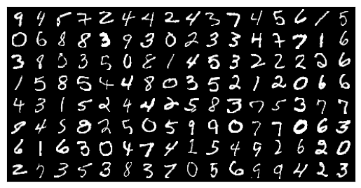
import torchvision
import matplotlib.pyplot as plt
import numpy as np

sample_idx = torch.randint(len(test_loader), size=(1,)).item()
dataiter = iter(test_loader)
for i in range(sample_idx): # randomly select a batch
    images, labels = next(dataiter)

# print test images
nrow = 16 # number of images per row
montage = torchvision.utils.make_grid(images, nrow=nrow)
plt.imshow(np.transpose(montage, (1, 2, 0)), cmap='gray')
plt.show()

# predict the labels
outputs = net(images.to(device))
_, predicted = torch.max(outputs, 1)
print("The predictions:\n", {predicted.reshape(batch_size // nrow, nrow)})

total = labels.size(0)
correct_rate = (predicted == labels.to(device)).sum().item() / total
print(f'Accuracy of the network on the 64 test images: {100 * correct_rate} %')
隨機選取的某個 batch 的數字影像 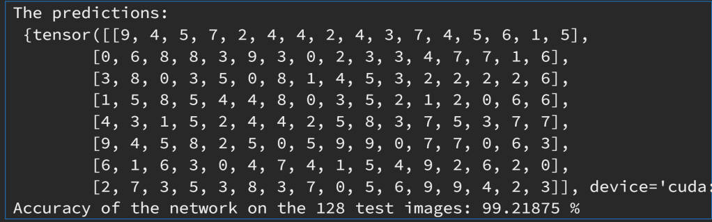
將左邊 128 張影像輸入訓練好之神經網路後的輸出預測值。
範例3:同上題,但更動 network 結構(Net2):留意 convolution 的 zero-padding=2,造成後續影像矩陣大小的變化。另外,network 的輸出有兩項,第二項作為其他用途。
class Net2(nn.Module):
    def __init__(self):
        super(Net2, self).__init__()
        self.conv1 = nn.Sequential(
            nn.Conv2d(
                in_channels=1,
                out_channels=16,
                kernel_size=5,
                stride=1,
                padding=2,
            ),
            nn.ReLU(),
            nn.MaxPool2d(kernel_size=2),
        )
        self.conv2 = nn.Sequential(
            nn.Conv2d(16, 32, 5, 1, 2),
            nn.ReLU(),
            nn.MaxPool2d(2),
        )
        # fully connected layer, output 10 classes
        self.out = nn.Linear(32 * 7 * 7, 10) # 32 * 7 * 7 is the size of the output of conv2
    def forward(self, x):
        x = self.conv1(x)
        x = self.conv2(x)
        # flatten the output of conv2 to (batch_size, 32 * 7 * 7)
        x = x.view(x.size(0), -1) # another way to flatten
        output = self.out(x)
        return output, x    # return x for visualization

device = "cuda:0" if torch.cuda.is_available() else "cpu"
print("Using {} device".format(device))

net2 = Net2().to(device)
print(net2)
Set up Loss function and optimizer
loss_func = nn.CrossEntropyLoss()
optimizer = optim.Adam(net2.parameters(), lr = 0.01)
Train the network
num_epochs = 15
def train(num_epochs, cnn, loaders):

    cnn.train()

    # Train the model
    total_step = len(loaders)

    for epoch in range(num_epochs):
        for i, (images, labels) in enumerate(loaders):

            b_x = images.to(device)   # batch x
            b_y = labels.to(device)   # batch y
            output = cnn(b_x)[0] # cnn output: get the first element of the returned tuple

            loss = loss_func(output, b_y)

            # clear gradients for this training step
            optimizer.zero_grad()

            # backpropagation, compute gradients
            loss.backward()
            # apply gradients
            optimizer.step()

            if (i+1) % 200 == 0:
                print ('Epoch [{}/{}], Step [{}/{}], Loss: {:.4f}'
                       .format(epoch + 1, num_epochs, i + 1, total_step, loss.item()))
                pass

        pass

    pass

train(num_epochs, net2, train_loader)
Evaluate the model on test data
def test():
    # Test the model
    net2.eval()
    with torch.no_grad():
        correct = 0
        total = 0
        for images, labels in test_loader:
            test_output, last_layer = net2(images.to(device))
            pred_y = torch.max(test_output, 1)[1]
            correct += (pred_y == labels.to(device)).sum().item()
            total += labels.size(0)
            # accuracy = (pred_y == labels.to(device)).sum().item() / float(labels.size(0))
            pass
    accuracy = correct / total
    print(f'Test Accuracy of the model on the {len(test_dataset)} test images: %.2f' % accuracy)

    pass
test()
Print 10 predictions from test data
sample = next(iter(test_loader))
imgs, lbls = sample
ground_truth = lbls[:10].numpy()
print("Ground truth:\n", ground_truth)

test_output, last_layer = net2(imgs[:10].to(device))
pred_y = torch.max(test_output, 1)[1]

print("Prediction:\n", pred_y.cpu().numpy())
練習:同上範例,將影像辨識資料改為 Yale Faces。CNN network 結構自訂。
練習:同上範例,資料改為手寫英文字母,共 26 個字母,3,700,000 張,每張 28×28。下載處:
https://www.kaggle.com/datasets/ashishguptajiit/handwritten-az